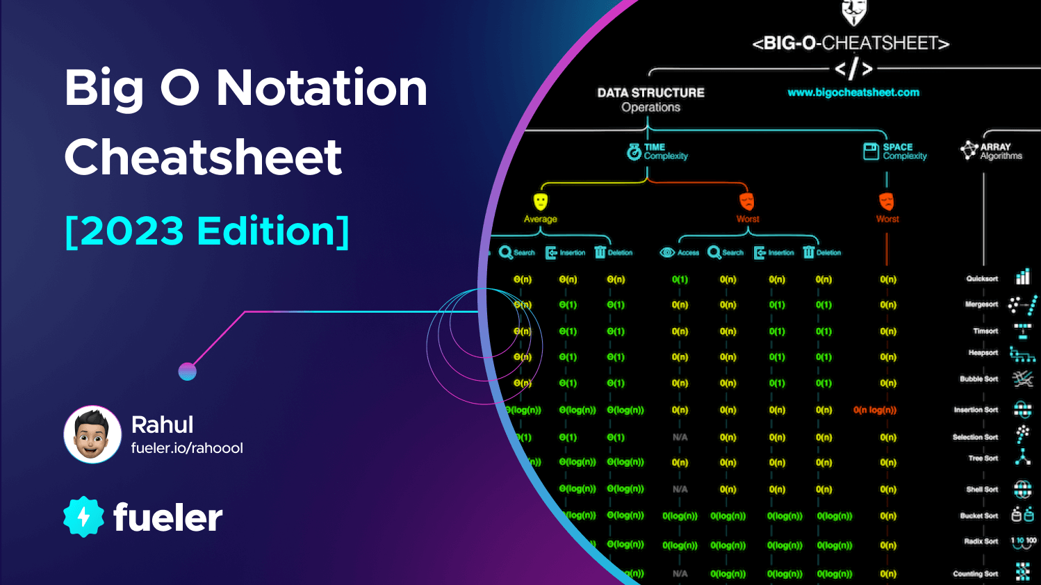
Ultimate Guide to Big O Notation in 2023 | A Comprehensive Cheatsheet

Rahul
04 Jan, 2023
If you're feeling a bit overwhelmed by the concept of Big O Notation and need a quick cheat sheet to help you understand it, then you've come to the right place! In this comprehensive guide, we'll give you all the tips and tricks you need to learn Big O Notation quickly and easily.
From the basics of Big O to some of its most common symbols, we'll cover what you need to know to help you in exams or just for coding at home.
Whether you're new to computer science or already have some coding skills, this cheat sheet will give you all the information you need about Big O Notation in one easy-to-follow guide.
So let's dive in!
Introduction to Big O Notation
If you're a programmer or studying computer science, you've probably heard of Big O notation. It's an important tool used in the analysis of algorithms and helps to determine the time complexity of a given software or program.
It's also essential for optimizing code and understanding how efficient your software performs.
An easy-to-follow Big O cheatsheet can help make understanding this complex concept simpler.
Big O notation is used to describe the runtime or space complexity of an algorithm.
A high-level description can be provided quickly for a simple algorithm without diving into every detail about how it works.
In Big O notation, two variables are used - the input size (n), and the amount of time it takes to execute (t). The notation gives us a way to compare algorithms based on their execution times - that is, to find out which algorithm is more efficient when dealing with different input sizes.
The purpose of our cheatsheet is to provide an overview of Big O notation, including its symbols, examples, and rules for determining time complexity.
To make things easier for those just starting out with Big O notation we'll provide examples using simple algorithms so you can better understand the concepts at hand.
Also included are resources to deepen your understanding should you want to explore further into this topic.
Basic Concepts
If you’ve been brushing up on algorithms and data structures, you may have heard of something called Big O Notation. But what is Big O Notation and why is it so important? Let's dive into this topic with a refresher on the basics to get you up to speed.
What Does "O" Stand For?
The "O" stands for the Greek letter "Omega," which essentially means infinite or unbounded. So when someone says something has an "O(n)" time complexity, they're talking about the runtime of an algorithm being relative to the size or quantity of input data (n).
What is Time Complexity?
Time complexity is a measure of how much time it takes for a computer algorithm to run and is usually expressed using Big O notation. It's a useful tool to help you understand how efficient certain algorithms are and how they scale with extra data.
Basically, the time complexity of an algorithm will determine how fast it can complete a task and how much memory it will require for larger datasets.
What is Space Complexity?
When it comes to understanding Big O Notation, one of the key elements that can define the performance of an algorithm is space complexity. Space complexity measures the amount of memory that an algorithm requires for it to execute, and is expressed in terms of the size of the input.
Understanding Asymptotic Behavior
Understanding Big O Notation requires understanding asymptotic behavior, which is when a function grows increasingly larger or smaller than some base value.
That increase can be taken at different rates—linear (O(n)), logarithmic (O(log n)), quadratic (O(n^2)), cubic (O(n^3))—and so on.
There are also common functions in Big O Notation that include constant functions (all runtimes are equal), exponential functions (runtime increases exponentially), and loglinear functions (when the runtime increases linearly with each additional input).
Now that you have a better understanding of the basic concepts behind Big O Notation, you're ready to explore this mathematical tool further!
Below this section, you will look at the key time and space complexities, explanations, and examples.
Big O Notation Cheatsheet
Learning Big O notation can be a challenge, and you may not have time to become an expert. That's why we've created this Big O Notation cheat sheet for you to bookmark and refer to as needed.
Let's quickly break it down:
Constant Time - O(1)
This is the fastest time complexity class — it means an algorithm takes the same amount of time regardless of the input size. A good example would be when you add two numbers together — it takes exactly the same amount of time whether you are adding 1 + 1 or 10^256 + 10^256.
Let's understand this from a simple example:
In the above example, the function add_numbers takes two integer inputs a and b and returns their sum. No matter what the values of a and b are, the function will always take the same amount of time to execute as it only performs a single operation of adding the two inputs together.
Logarithmic Time - O(log n)
This is a bit slower than constant time, but still pretty fast. Put simply, it means that if your input size doubles, the algorithm will only take one more step to finish which is amazing compared to other complexity classes.
An example would be searching a sorted array — as you iterate through it, the search space gets halved after each check since “binary search” divides and conquers approach is used.
def binary_search(arr, target):
    left, right = 0, len(arr) - 1
    while left <= right:
        mid = (left + right) // 2
        if arr[mid] == target:
            return mid
        elif arr[mid] < target:
            left = mid + 1
        else:
            right = mid - 1
    return -1
In the above example, the binary search algorithm takes a sorted array "arr" and a target value "target" as input. It initializes two pointers "left" and "right" to the beginning and end of the array respectively, and then repeatedly divides the search space in half by computing the midpoint "mid".
If the target value is found at the midpoint, the function returns the index of the midpoint. If the target value is less than the midpoint, the function continues the search on the left half of the array by updating the "right" pointer.
Otherwise, the function continues the search on the right half of the array by updating the "left" pointer.
Linear Time - O(n)
This complexity type is actually quite slow compared to the previous two, because here your time for computation grows proportionally with your input size — i.e., double your inputs and the algorithm will take twice as much time.
An example would be finding something in an unsorted array — each iteration takes longer until you find what you’re looking for.
def find_element(my_list, element):
    for num in my_list:
        if num == element:
            return True
    return False

my_list = [3, 7, 1, 9, 5, 2, 8]
print(find_element(my_list, 9)) # Output: True
print(find_element(my_list, 4)) # Output: False
In this example, the function find_element takes a list my_list and an element element as input. It iterates through the list and checks each element to see if it matches the desired element. If it finds a match, it returns True. If it reaches the end of the list without finding a match, it returns False.
The time complexity of this algorithm is O(n), as the number of iterations (that is the time it takes to find the element) grows proportionally with the size of the list.
Linearithmic Time - O(n log n)
Linearithmic time is an algorithm that takes a certain amount of time to run but scales logarithmically with the size of the data input. This means that when you double your data set, the algorithm only takes twice as long to run.
Let's say you have an unsorted list of numbers and you want to sort them in ascending order using the Merge Sort algorithm.
Merge Sort has a time complexity of O(n log n) in the worst-case scenario, meaning that as the size of the input list (n) increases, the time taken to sort the list increases logarithmically.
def merge_sort(arr):
    if len(arr) <= 1:
        return arr

    mid = len(arr) // 2
    left = arr[:mid]
    right = arr[mid:]

    left = merge_sort(left)
    right = merge_sort(right)

    return merge(left, right)

def merge(left, right):
    result = []
    i = 0
    j = 0

    while i < len(left) and j < len(right):
        if left[i] < right[j]:
            result.append(left[i])
            i += 1
        else:
            result.append(right[j])
            j += 1

    result += left[i:]
    result += right[j:]

    return result
In this example, when we call the merge_sort function on an unsorted list, it will divide the list into smaller sublists, sort them recursively using merge_sort, and then merge them back together using the merge function.
The time complexity of Merge Sort is O(n log n) because the algorithm divides the input list into halves repeatedly until each sublist contains only one element (which takes O(log n) time), and then merges the sublists together in a linear time of O(n) for each level of the recursion, resulting in a total time complexity of O(n log n).
As the size of the input list (n) increases, the time taken to sort the list increases logarithmically.
Exponential time - O(2^n)
Exponential Time (O(2^n)) is when the time required to complete an algorithm doubles with each increase in input size.
This means that the growth rate of this type of algorithm is exponential—for every extra item in its input, the time it needs more than doubles!
def fibonacci(n):
    if n <= 1:
        return n
    else:
        return fibonacci(n-1) + fibonacci(n-2)
In the above example, we have a recursive function that calculates the nth Fibonacci number. The function makes two recursive calls for each value of n. As a result, the time required to calculate the nth Fibonacci number doubles with each increase in n.
Factorial time - O(n!)
Factorial Time (O(n!)) refers to a type of algorithm which requires processing all possible combinations of a set.
This means that the input size increases exponentially—for every extra item added, there are more unique combinations possible, and thus more calculation required.
Let's say you have a list of numbers [1, 2, 3], and you want to find all possible permutations of the list.
import itertools

def find_permutations(lst):
    permutations = []
    for permutation in itertools.permutations(lst):
        permutations.append(permutation)
    return permutations
If we call this function with the list [1, 2, 3], it will return a list of all possible permutations of that list: [(1, 2, 3), (1, 3, 2), (2, 1, 3), (2, 3, 1), (3, 1, 2), (3, 2, 1)].
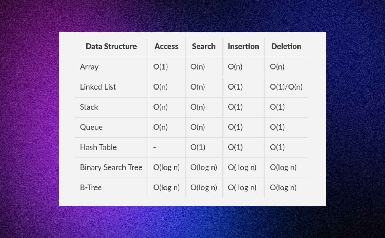
Data Structure Complexity Chart
- Access means accessing an element at a given index
- Search means finding an element with a given key
- Insertion means adding a new element to the data structure
- Deletion means removing an element from the data structure
- n is the number of elements in the data structure
- m is the length of the key being searched in the Trie
- "-" means the operation is not applicable or not defined for that data structure.
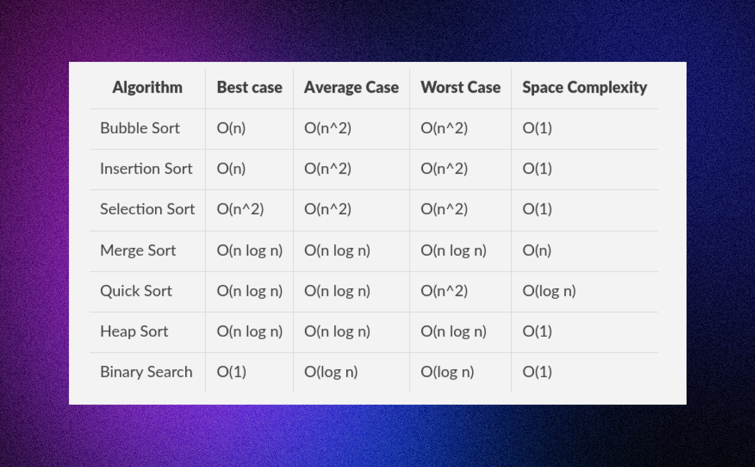
Algorithm Complexity Chart
When talking about Big O Notation, it's important to differentiate between best-case, average-case and worst-case scenarios.
Best Case Scenario: The best-case scenario is when a given algorithm takes the least amount of time to complete it’s task. This means it has the most optimal performance.
Average Case Scenario: The average-case scenario is when an algorithm completes its task in an expected amount of time – neither too fast nor too slow. It's neither the best nor worst case, but rather a combination of different scenarios.
Worst Case Scenario: The worst-case scenario is when a given algorithms takes the most amount of time to complete its task. This means that it has the least optimal performance. This is important to consider because algorithms are typically designed with worst-case scenarios in mind, so they run efficiently even under unfavorable conditions.
When talking about Big O Notation, it's important to understand each scenario and determine which one best suits your needs – as this can make a huge difference in terms of performance!
Which one to focus on? Time Complexity or Space Complexity?
The answer depends on your use case. If you're dealing with a real-time system like a video game with strict time constraints then it's important to focus on time complexity; if you're concerned about memory usage then focus on space complexity.
Ultimately, it depends on your underlying needs — knowing when to focus on each type of Big O notation can help you create better algorithms for your use cases and optimize your codebase.
Conclusion
In summary, Big O notation is an essential tool for any developer or data scientist. It's a simple way of identifying the time complexity of an algorithm, and is incredibly useful when analyzing algorithms to see which perform best. It can also be used to evaluate data structures and determine the best one to use for a particular application.
Having a solid understanding of Big O notation will help you become a better programmer and data scientist. With the cheatsheet in this article, you can look up the complexity of any algorithm or data structure, and improve your coding.
So, don't miss the chance to become a pro and build algorithms for complex data structures with the help of Big O notation cheatsheets.
What should you do next?
You've read the article. Now turn your skills into proof of work and unlock more opportunities.
Build your proof of work portfolio
Create a clean portfolio with projects, assignments, resumes, and AI stack details that companies actually want to see.
Create your Fueler portfolio →Apply through assignments, not resumes
Stand out by solving real tasks from companies hiring on Fueler.
Explore assignments →Get discovered by companies
Make your work public and let recruiters discover your skills through actual projects instead of keywords.
Get discovered →